A while ago I had a simple-sounding question to answer: across a large pile of transactional emails, which senders send which kinds of messages? How many “Your order has shipped” emails does each merchant send, compared with order confirmations, delivery notices and promotions?

The email headers sat in Amazon S3 as gzipped JSON, and I did the analysis in an Apache Zeppelin notebook running Spark. The code was short. Understanding why some versions of it took seconds and others took minutes was the interesting part, and it’s a good way to learn how Spark actually works.

For this post I rebuilt the same analysis on 3 million synthetic email headers (fictional senders, no real data) and ran it on Spark 3.5 on my laptop. Every plan, task count and timing below is real output from that run.

The question and the data

Each email is one JSON line with a few header fields:

{"message_id": "<0000002a@mail.example>", "date": "2025-09-15T08:12:44Z",
 "from": "Acme Store <no-reply@acme-store.example>",
 "to_hash": "9f2c1e7a4b3d8c06", "subject": "Your order #48213 has shipped"}

The files are partitioned by day, which is the usual layout for event data on S3:

s3://your-bucket/email-headers/
  dt=2025-09-01/part-00000.json.gz
  dt=2025-09-01/part-00001.json.gz
  ...
  dt=2025-09-30/part-00119.json.gz

A note on privacy, because email data is personal data. The analysis only needs who sent it (a business sender domain) and the subject line. It never needs message bodies or recipient addresses, so recipients are stored only as a hash, and the output is aggregated counts per sender. If you do this kind of analysis for real, keep it that way: read the minimum columns and never export row-level results.

The notebook

In Zeppelin, a note is a list of paragraphs, and each one starts with an interpreter such as %pyspark or %sql. Both share the same Spark session, so a view registered in Python can be queried in SQL right after.

The first paragraph does all the work: extract the sender domain from the From header, classify the subject into a type, and count:

%pyspark
from pyspark.sql import functions as F, types as T

schema = T.StructType([
    T.StructField("message_id", T.StringType()),
    T.StructField("date", T.StringType()),
    T.StructField("from", T.StringType()),
    T.StructField("to_hash", T.StringType()),
    T.StructField("subject", T.StringType()),
])

headers = spark.read.schema(schema).json("s3://your-bucket/email-headers/")

CONFIRMED = (r"order confirmation|thanks for your order"
             r"|received your order|order is confirmed")
PROMOTION = r"% off|\bsale\b|last chance|new arrivals"

subject = F.lower(F.col("subject"))
email_type = (
    F.when(subject.rlike(r"\bdelivered\b"), "delivered")
     .when(subject.rlike(r"\bshipped\b|on its way"), "shipped")
     .when(subject.rlike(CONFIRMED), "order confirmation")
     .when(subject.rlike(PROMOTION), "promotion")
     .otherwise("other")
)
sender = F.lower(F.regexp_extract("from", r"@([\w.-]+)>?\s*$", 1))

summary = (
    headers
    .withColumn("sender", sender)
    .withColumn("email_type", email_type)
    .groupBy("sender", "email_type")
    .count()
)
summary.createOrReplaceTempView("email_types")

Two details in the classifier matter more than they look. The order of the when clauses is the priority order, so “Delivered: order #123” is not also counted as a confirmation. And \bshipped\b is a whole word on purpose: a lazy contains("ship") would count “Last chance: free shipping ends tonight” as a shipping notice.

The second paragraph is plain SQL, and Zeppelin turns the result into a chart with one click:

%sql
SELECT sender, email_type, count
FROM email_types
ORDER BY count DESC

Here is the result for the six largest senders and the long tail of smaller shops:

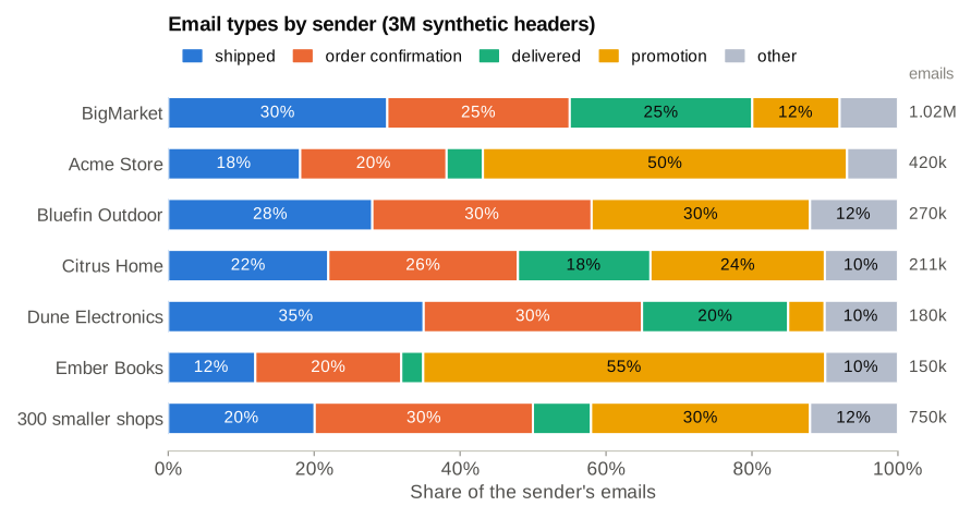
Synthetic data with fictional senders. The patterns are the kind you see in real mail: some senders mostly send promotions, and some never send a “delivered” email at all.

So that’s the answer. Now let’s look at what Spark did to get it.

Who does what: driver, cluster manager, executors

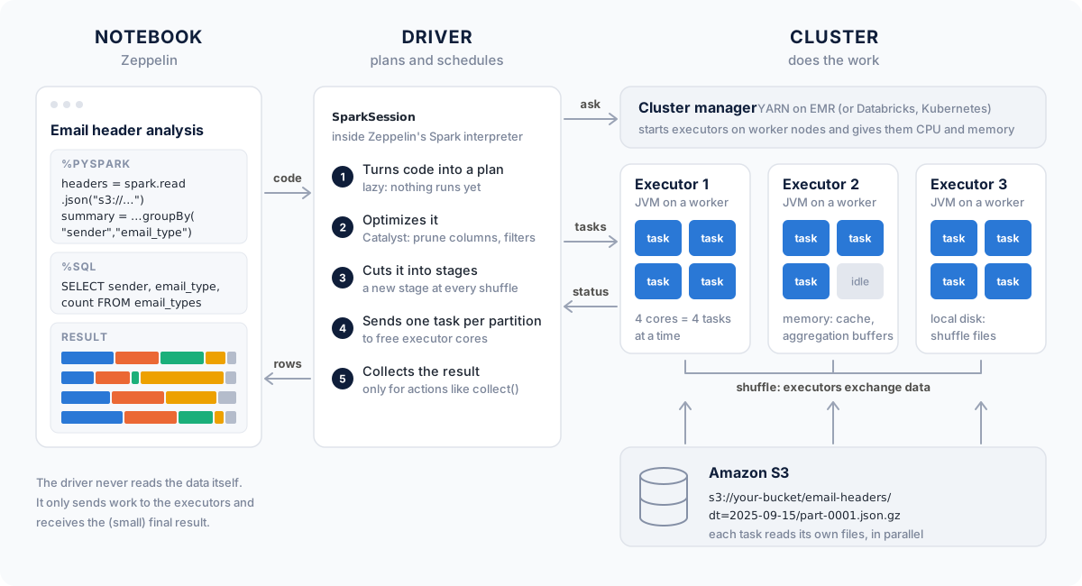
A Spark application has three kinds of parts:

• The driver holds your SparkSession. It turns your code into a plan, splits the plan into tasks and schedules them. In Zeppelin, the driver usually lives inside the Spark interpreter process, which is why restarting the interpreter throws away your session, your cached data and your temp views.
• The cluster manager (YARN on Amazon EMR, Kubernetes, or the Databricks control plane) starts executors on worker nodes and gives them CPU and memory.
• Executors are JVM processes that do the real work. Each executor core runs one task at a time, and each task processes one partition of the data.

The driver never reads the email files itself. Executors read them straight from S3, in parallel, and only the small final result travels back to the driver. That’s also why collect() on a large DataFrame is dangerous: it pulls every row into the driver’s memory. Zeppelin protects you a little here, because its table display only shows the first 1,000 rows by default (zeppelin.spark.maxResult).

Lazy evaluation: nothing runs until an action

Spark operations come in two kinds:

• Transformations such as read, withColumn, filter and groupBy only describe what you want. They return instantly.
• Actions such as collect, count, show and write need a result, so they start a job.

In my run, building the whole summary DataFrame took 0.03 seconds and started zero jobs. Calling summary.collect() took 2.6 seconds and did all the work.

There is one surprise in here that shows up in almost every notebook. My first version read the files without a schema:

headers = spark.read.json("s3://your-bucket/email-headers/")   # no schema

That line, which looks like a transformation, immediately ran two jobs that took 6.2 seconds, more than twice as long as the real query:

Job	What it did	Tasks
0	List 3,600 files in parallel	3,600
1	Read all 85.6 MB of data to infer the JSON schema	113

To infer a schema, Spark has to read the data, so with JSON or CSV you pay for an extra full scan before your query even starts. On S3 with real data volumes, that can be minutes. Passing an explicit schema, as in the notebook above, makes the read lazy again. (Parquet stores its schema in the files, so it doesn’t have this problem.)

One action, one job, two stages, 118 tasks

When collect() runs, the driver turns the plan into stages and tasks. Here’s the physical plan Spark printed after the query ran:

AdaptiveSparkPlan isFinalPlan=true
+- == Final Plan ==
 *(2) HashAggregate(keys=[sender, email_type], functions=[count(1)])
 +- AQEShuffleRead coalesced
    +- ShuffleQueryStage 0
       +- Exchange hashpartitioning(sender, email_type, 200)
          +- *(1) HashAggregate(keys=[sender, email_type],
                                functions=[partial_count(1)])
             +- *(1) Project [lower(regexp_extract(from, ...)) AS sender,
                              CASE WHEN RLIKE(...) ... END AS email_type]
                +- FileScan json [from,subject,dt]
                     PartitionFilters: [], PushedFilters: [],
                     ReadSchema: struct<from:string,subject:string>

The full output is longer. I trimmed expression IDs, the regex details and the file path, and re-wrapped long lines. Read it from the bottom up, and look for the Exchange. That’s the shuffle, and every shuffle is a stage boundary:

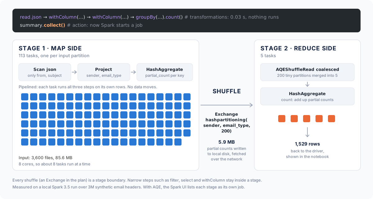
Stage 1 (map side) ran 113 tasks. Each task read its share of the files and ran the scan, the projection and a partial count back to back. These steps are narrow: every output row depends on one input row, so they can be pipelined inside one task with no data movement. The *(1) in the plan marks operators that Spark fused into a single generated function (whole-stage code generation). Notice the ReadSchema too: Spark only parses from and subject, because those are the only columns the query uses.

The shuffle sent each task’s partial counts to the partition that owns each (sender, email_type) key. Because of the partial aggregation, 3 million rows became just 5.9 MB of shuffle data. This is the same map-side combiner trick I explained in How MapReduce Works.

Stage 2 (reduce side) would normally have 200 tasks, the default spark.sql.shuffle.partitions. But with adaptive query execution (AQE, on by default since Spark 3.2), Spark saw that 200 partitions would be tiny and coalesced them into 5 (AQEShuffleRead coalesced). Five tasks added up the partial counts and returned 1,529 rows, one per sender and type.

One quirk to know when you open the Spark UI: with AQE, each stage is submitted as its own job, so this one query shows up as two jobs, and the second one lists the map stage again as skipped, meaning its shuffle output was reused rather than recomputed.

Where the task count comes from

The number of tasks in the first stage is the number of input partitions, and that’s decided by how your files are laid out. This is where most real-world Spark performance problems start, and S3 makes them worse.

For file sources, Spark packs files into partitions of up to spark.sql.files.maxPartitionBytes (128 MB by default), counting each file as at least spark.sql.files.openCostInBytes (4 MB) so that thousands of tiny files don’t each become a task. Large splittable files are cut into several partitions. But gzip is not splittable: a .json.gz file must be decompressed from the start, so one gzip file is always read by one task, no matter how big it is.

To see the effect, I wrote the same 3 million rows in four layouts and ran the same query on each:

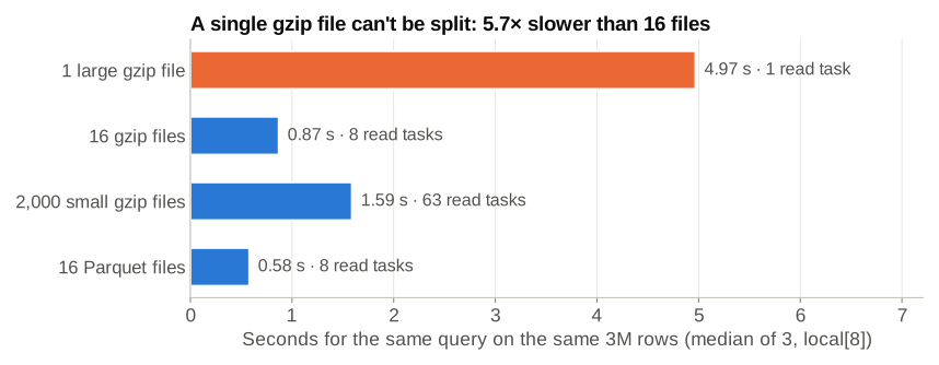
Local run with 8 cores, median of three runs after a warm-up. On S3 the gaps are larger, because every file is a separate request with its own latency.

• One large gzip file: one task did all the work while the other seven cores sat idle. 5.7× slower than 16 files. On a cluster with hundreds of cores, the gap is far bigger.
• 2,000 small files: Spark packed them into 63 tasks, but opening and decompressing each file still has a cost, so it was almost 2× slower than 16 files of the same data. On S3, each file also means a GET request and more listing work for the driver.
• Parquet: fastest even though its files were larger on disk, because Spark only read the two columns it needed.

And here’s an honest confession: the “realistic” dataset in this post ended up with 3,600 small files, by accident. I wrote it with repartition(120) followed by partitionBy("dt"). Every one of the 120 tasks held rows from all 30 days, so each task wrote one file into every day folder: 120 × 30 = 3,600 files of about 24 KB each. It’s one of the most common ways small files get created. Repartition by the partition column instead, so each task writes to only one folder:

(df.repartition("dt")            # rows for one day end up in one task
   .write.partitionBy("dt")
   .json("s3://your-bucket/email-headers/"))

Partitioning by date also pays off on the read side. Filtering on dt lets Spark skip whole folders before it opens a single file (PartitionFilters in the plan). Analyzing one day instead of the month took 0.29 seconds, 8 tasks and 2.9 MB of input.

Reading the Spark UI

Everything above came from the Spark UI and its REST API, and it’s the first place to look when a notebook paragraph is slow. In Zeppelin you can open it from the link shown on a running Spark paragraph, or from the cluster’s resource manager on EMR. What to check:

• Jobs tab: an unexpected job, like schema inference or a count() you forgot about, is wasted time.
• Stages tab: the number of tasks (too few means idle cores; tens of thousands means too many small files), Input size, and Shuffle Read / Shuffle Write. A big shuffle write is the usual cause of a slow query.
• Task summary within a stage: if the max task duration is far above the median, you have skew. One very big sender (like “BigMarket” here, a third of all mail) is a classic hot key in joins and window functions.
• SQL tab: the same plan as EXPLAIN, with row counts and sizes on every operator.

A checklist for Spark on S3

1. Give JSON and CSV reads an explicit schema. Otherwise you pay for a full scan just to read the data.
2. Select only the columns you need, and filter on partition columns early. Spark can push both down to the scan.
3. Avoid one big gzip file. Use many files of roughly 128 MB to 1 GB, or a splittable format.
4. Avoid thousands of tiny files. Repartition by the partition column before partitionBy, or compact small files in a regular job.
5. Prefer Parquet (or Delta, Iceberg) for anything you query more than once. Convert raw JSON once, and query the columnar copy.
6. Keep collect() for small results. Aggregate on the cluster first, then bring back the summary.
7. Leave AQE on, and look at the Stages tab before you start tuning spark.sql.shuffle.partitions by hand.

Takeaways

• The driver plans and schedules; executors do the work, one task per partition per core.
• Transformations are lazy, actions run jobs, but reading JSON or CSV without a schema quietly runs jobs of its own.
• A job is cut into stages at every shuffle. Narrow steps are pipelined inside a stage; an Exchange in the plan means data crosses the network.
• The number of tasks comes from your file layout, so file size, file count and format often matter more than any Spark setting.

How the numbers were made: a PySpark script generated 3 million synthetic headers from 306 fictional senders (all on the reserved .example domain), wrote them in the layouts above, and ran the query on Spark 3.5.3 in local mode with 8 cores. Task counts, shuffle sizes and timings come from the Spark UI’s REST API. You can reproduce all of it on a laptop with Java 17 and pip install pyspark.

If this was useful, the companion post How MapReduce Works covers the map, shuffle and reduce pattern that Spark’s stages are built on.

More from PipePrompt

• Migrating Production Spark Pipelines off Databricks: What Broke, and How We Proved the Data Matched

  Oct 13, 2026 · databricks, spark, migration, iceberg, data engineering, ai

  Moving dozens of Spark pipelines off Databricks: silent SQL translation bugs, hidden state, stale inputs, hash-based parity checks, and how AI helped.

• How MapReduce Works: From Hadoop Word Count to GROUP BY in Spark SQL

  Oct 11, 2026 · hadoop, mapreduce, spark, data engineering, databricks

  How Hadoop MapReduce works, with diagrams, a runnable word count, and how a GROUP BY on Databricks or WeData turns into map, shuffle and reduce.

• Building an Automated Data Quality Framework: Rules, Trend Detection, and LLM False-Alarm Filtering

  Oct 28, 2025 · data quality, data engineering, llm, python

  How to build automated data quality checks: rule-based checkers, regression trend detection, ID pattern analysis, and LLM false-alarm filtering.