Few teams write raw Hadoop MapReduce jobs anymore. But every time you run a GROUP BY or a JOIN on Databricks, on Tencent Cloud WeData, or on any other big data platform, the engine underneath still follows the same three-step pattern Hadoop made famous: map, shuffle, reduce.

Once you understand that pattern, a lot of “why is this query slow?” questions answer themselves. This post explains how MapReduce works with diagrams and a word count you can run on your laptop, then follows a real-world style SQL query through the same three steps.

The idea in one picture

MapReduce splits a big job into many small, independent pieces of work:

1. Map: each worker reads its own chunk of the input and emits (key, value) pairs.
2. Shuffle: pairs with the same key are moved to the same worker.
3. Reduce: each worker combines all the values for each of its keys.

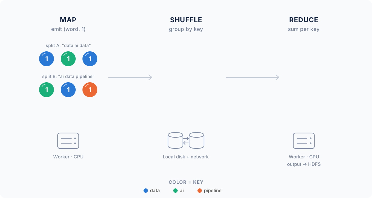
Each color is one key. Map emits a 1 for every word, the shuffle brings equal keys together, and reduce adds them up.

The trick is that map and reduce never need to talk to each other. Map tasks run in parallel on as many machines as you have, and so do reduce tasks. The only coordination happens in the shuffle, which is why the shuffle is also where most of the cost is.

Word count, step by step

Word count is the “hello world” of MapReduce. Take two tiny input splits, data ai data and ai data pipeline, and count how often each word appears:

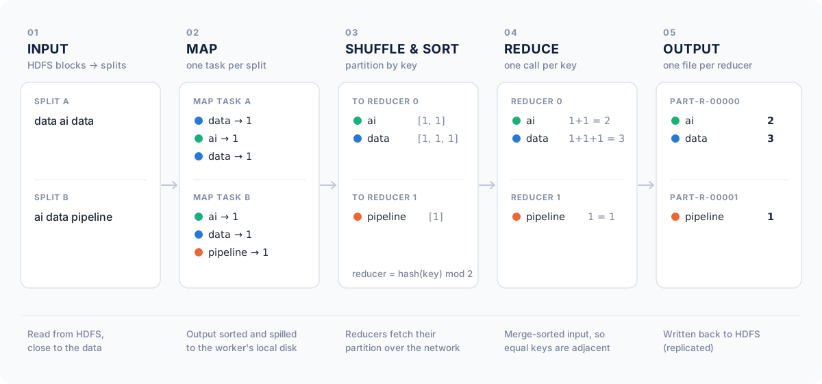
Here is what happens at each step in Hadoop:

1. Input splits. Files in HDFS are stored as blocks (128 MB by default). Each block usually becomes one input split, and each split gets its own map task. The scheduler tries to run that task on a machine that already holds the block (data locality), so the input doesn’t have to cross the network.
2. Map. The map function turns each record into key-value pairs. For word count, every word becomes (word, 1).
3. Partition, sort and spill. Map output goes into an in-memory buffer (100 MB by default). Each pair is assigned to a reducer with hash(key) mod number_of_reducers, then sorted by key. When the buffer fills up, it’s spilled to the worker’s local disk, not to HDFS.
4. Shuffle. Each reducer fetches its partition from every map task over the network, and merge-sorts the pieces. Because the input is sorted, all values for the same key arrive next to each other.
5. Reduce. The reduce function is called once per key with all its values: data → [1, 1, 1] becomes data 3.
6. Output. Each reducer writes one file (part-r-00000, part-r-00001, …) back to HDFS, where it’s replicated like any other file.

Try it yourself

Hadoop Streaming lets you write the mapper and reducer in any language that reads stdin and writes stdout. Here is a complete word count in Python.

mapper.py:

#!/usr/bin/env python3
"""Map: read raw text, emit one "word<TAB>1" line per word."""
import re
import sys

for line in sys.stdin:
    for word in re.findall(r"[a-z']+", line.lower()):
        print(f"{word}\t1")

reducer.py:

#!/usr/bin/env python3
"""Reduce: input arrives sorted by key, so all counts for a word are adjacent."""
import sys

current, total = None, 0
for line in sys.stdin:
    word, count = line.rstrip("\n").split("\t", 1)
    if word != current:
        if current is not None:
            print(f"{current}\t{total}")
        current, total = word, 0
    total += int(count)

if current is not None:
    print(f"{current}\t{total}")

You don’t need a cluster to see it work. On a single machine, the Unix sort command plays the role of the shuffle:

$ printf 'data ai data\nai data pipeline\n' > input.txt
$ cat input.txt | python3 mapper.py | sort | python3 reducer.py
ai	2
data	3
pipeline	1

On a real cluster, the same two scripts run as a distributed job:

hadoop jar $HADOOP_HOME/share/hadoop/tools/lib/hadoop-streaming-*.jar \
  -files mapper.py,reducer.py \
  -mapper "python3 mapper.py" \
  -combiner "python3 reducer.py" \
  -reducer "python3 reducer.py" \
  -input /data/books \
  -output /data/wordcount

Notice the -combiner line. It reuses the reducer as a combiner, which brings us to the most important optimization in MapReduce.

The combiner: reduce before you shuffle

A combiner runs the reduce logic on each map task’s own output before it is shuffled. Instead of sending data 1 three times, map task A sends data 2 once. This works whenever the reduce operation is associative and commutative, like sum, count, min and max.

The effect on shuffle volume is large, because real text (and most real data) repeats the same keys many times:

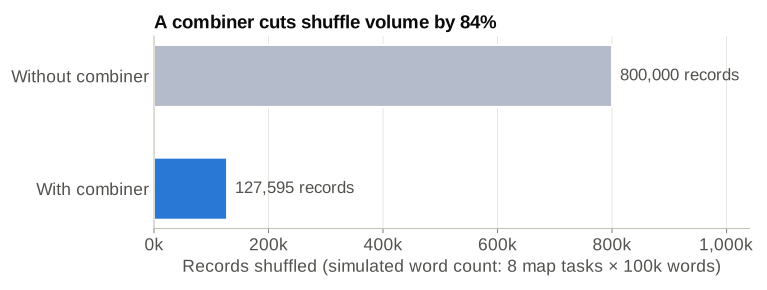
Simulated word count with a realistic, Zipf-like word distribution. Common words like “the” are counted locally first, so each map task sends each distinct word only once.

What runs where: HDFS, YARN and fault tolerance

A Hadoop cluster has two layers working together:

• HDFS stores the data. A NameNode keeps track of which blocks make up each file and where they are; DataNodes store the blocks, with 3 replicas by default.
• YARN runs the computation. The ResourceManager hands out CPU and memory across the cluster, a NodeManager on each machine launches containers, and each job gets an ApplicationMaster that schedules its map and reduce tasks.

This design is what makes MapReduce robust on cheap hardware:

• Failed tasks are retried on another machine (up to 4 attempts by default). Because map tasks only read their input split and write local output, re-running one is safe.
• Slow tasks get a backup. With speculative execution, if one task is much slower than its peers, a copy starts elsewhere and whichever finishes first wins.
• Lost map output is recomputed. If a node dies after its map tasks finish but before reducers fetch the output, those map tasks simply run again.

From MapReduce to SQL: a GROUP BY on Databricks or WeData

Now the part that matters day to day. Take a typical reporting query:

SELECT country, COUNT(*) AS orders
FROM sales.orders
WHERE order_date >= '2025-01-01'
GROUP BY country

On Databricks this runs on Spark. On Tencent Cloud WeData, the SQL in a data development task is handed to an execution engine underneath, such as Spark or Hive on EMR, or Spark on DLC. Either way, the engine turns the query into the same map, shuffle and reduce steps:

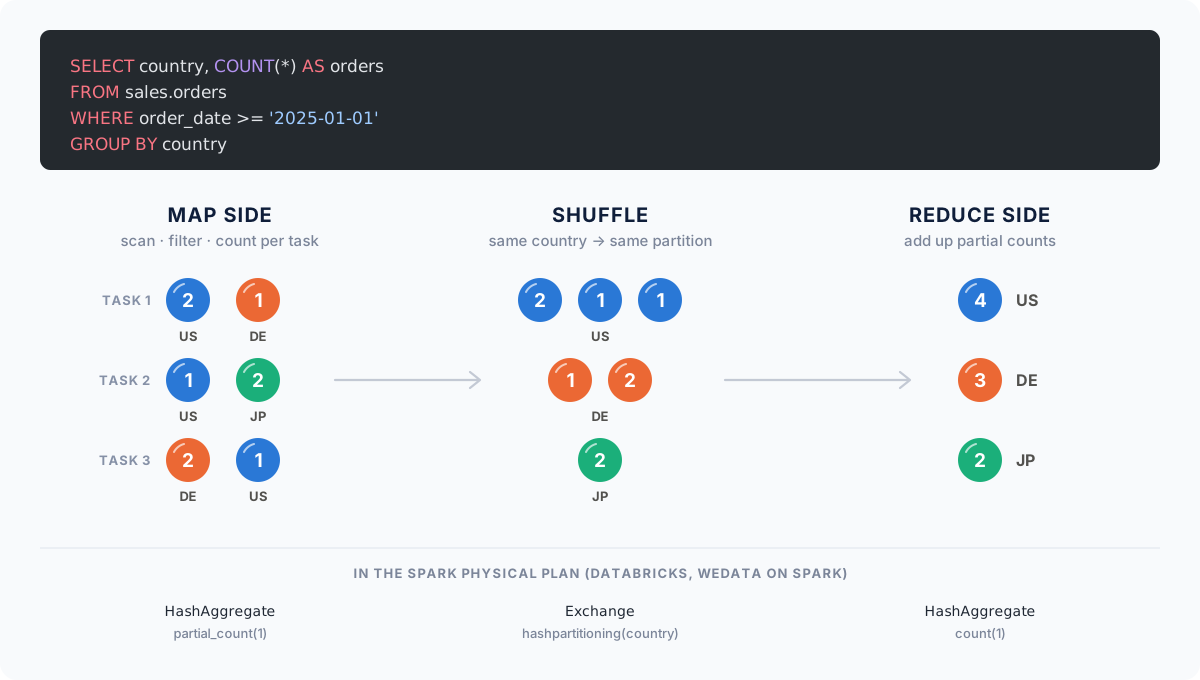
You can see this directly in the query plan. Running EXPLAIN on the query in Spark gives a plan like this (simplified: expression IDs and file details removed). Read it from the bottom up:

== Physical Plan ==
AdaptiveSparkPlan isFinalPlan=false
+- HashAggregate(keys=[country], functions=[count(1)])                  <- reduce
   +- Exchange hashpartitioning(country, 200)                            <- shuffle
      +- HashAggregate(keys=[country], functions=[partial_count(1)])     <- map + combiner
         +- Project [country]
            +- Filter (isnotnull(order_date) AND (order_date >= 2025-01-01))
               +- FileScan parquet sales.orders [country, order_date]

• FileScan + Filter + Project is the map side: each task reads its own files and keeps only the rows and columns it needs.
• HashAggregate ... partial_count is the combiner: each task counts its own rows per country before anything leaves the machine.
• Exchange hashpartitioning(country, 200) is the shuffle: partial counts are sent so that each country lands in exactly one of 200 partitions (Spark’s default for spark.sql.shuffle.partitions).
• The top HashAggregate ... count is the reduce side: one final count per country.

If your WeData task runs on Hive with the MapReduce engine, EXPLAIN is even more literal: the plan is printed as a Map Operator Tree and a Reduce Operator Tree.

What Spark changed, and what it didn’t

Spark is much faster than classic Hadoop MapReduce for most workloads, mainly because a multi-step query runs as one job with several stages, and intermediate results don’t have to be written to HDFS between steps. But the shuffle is still there: every Exchange in a Spark plan is a stage boundary, and shuffle data is still written to local disk and fetched over the network.

That’s why, in the Spark UI on Databricks, the Shuffle Read and Shuffle Write columns of the Stages tab are usually the first place to look when a query is slow. For a step-by-step look at jobs, stages and tasks on a real query, see How Spark Works.

Making shuffles cheaper in practice

Everything that makes MapReduce fast or slow carries over to modern SQL engines. A few habits pay off on any platform:

1. Shrink the data before the shuffle. Filter early, select only the columns you need, and filter on partition columns so whole files are skipped. Less map output means less shuffle.

2. Let the engine pre-aggregate. Spark does partial aggregation automatically for COUNT, SUM, MIN and MAX, and Hive does it by default (hive.map.aggr=true). Aggregations that can’t be combined, like COUNT(DISTINCT ...) or collect_list, shuffle much more data.

3. Avoid the shuffle entirely for small tables. When you join a large table with a small one, a broadcast join copies the small table to every worker instead of shuffling both sides. Spark does this automatically below spark.sql.autoBroadcastJoinThreshold (10 MB by default), and you can force it with a hint:

SELECT /*+ BROADCAST(c) */ o.order_id, c.country_name
FROM sales.orders o
JOIN ref.countries c ON o.country = c.country_code

4. Watch for skew. The shuffle sends every row with the same key to the same reducer. If one key is much bigger than the others, one task ends up doing most of the work while the rest of the cluster waits:

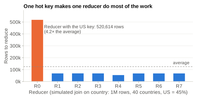
Simulated join on a skewed key. The whole stage finishes only when the slowest task does.

In the Spark UI, skew shows up as a stage where the max task duration is far above the median. For aggregations like the GROUP BY above, partial aggregation already neutralizes most of it. For joins, enable adaptive query execution (on by default since Spark 3.2), which splits oversized partitions automatically when spark.sql.adaptive.skewJoin.enabled is true. If that’s not enough, salt the hot key: add a random suffix to spread it over several partitions, then aggregate again.

Takeaways

• MapReduce is three steps: map (parallel, local), shuffle (group by key across the network), reduce (combine per key).
• The shuffle is the expensive part. Most optimizations, from combiners to broadcast joins, are ways to send less data through it.
• Modern engines such as Spark on Databricks, or the Spark and Hive engines behind WeData, still compile GROUP BY and JOIN into the same pattern. You can see it in every Exchange of a query plan.
• When a big query is slow, look at shuffle size and task skew before anything else.

More from PipePrompt

• Migrating Production Spark Pipelines off Databricks: What Broke, and How We Proved the Data Matched

  Oct 13, 2026 · databricks, spark, migration, iceberg, data engineering, ai

  Moving dozens of Spark pipelines off Databricks: silent SQL translation bugs, hidden state, stale inputs, hash-based parity checks, and how AI helped.

• How Spark Works: Jobs, Stages and Tasks, Explained with an Email Header Analysis

  Oct 11, 2026 · spark, zeppelin, aws, data engineering, performance

  How Apache Spark runs your code: driver, executors, jobs, stages, tasks and the shuffle, shown with a Zeppelin notebook that analyzes email headers on S3.

• Building an Automated Data Quality Framework: Rules, Trend Detection, and LLM False-Alarm Filtering

  Oct 28, 2025 · data quality, data engineering, llm, python

  How to build automated data quality checks: rule-based checkers, regression trend detection, ID pattern analysis, and LLM false-alarm filtering.