Manual data quality review doesn’t scale. Once a pipeline produces millions of records a day across hundreds of fields, nobody can eyeball enough of it to catch problems early, and the issues that slip through are the ones downstream teams notice first.

This post describes the design of an Auto Data Quality (Auto DQ) framework I worked on for a high-volume extraction pipeline. Its job is to catch tagging and extraction errors automatically, cut manual review effort, and keep accuracy high. Company names and proprietary metrics have been removed; what’s left is the architecture and the algorithms, with small Python examples you can adapt.

Architecture overview

The framework rests on three pillars:

1. Rule-based checkers that catch known classes of errors in individual records.
2. A data trends monitor that catches problems only visible over time.
3. False alarm control, which filters the output of the first two so humans only review what matters.

graph TD
    A[Raw Data] --> B(Rule-Based Checkers)
    A --> C(Data Trends Monitor)
    B --> D{False Alarm Control}
    C --> D
    D -->|Similarity / LLM Filter| E[Filtered Reports]

1. Rule-based checkers

The system runs hundreds of rules across multiple domains and fields. A few representative families:

• Mail body checker: finds values that exist in the source text but were never extracted. For example, if no total price was tagged, it looks for a currency symbol and digits near the word “total” in the original email body.
• Duplicate order checker: flags records that match on key fields such as a unique GUID, total price, product name, purchase date, and email timestamp.
• Price checker: catches pricing anomalies such as missing tags, wrong tags (for example, TotalPrice far larger than the sum of item prices plus shipping), and impossible quantities (qty > 10000).
• Other checkers: long-tail cases, common-sense validations, and custom checks added on demand.

Rules are cheap, fast, and easy to explain, which makes them the right first line of defense. Their weakness is noise, which is what false alarm control (section 4) is for.

2. Trend detection on timeline data

Some problems are invisible in any single record. A field whose fill rate slowly drops from 95% to 60% over three weeks passes every rule, every day. To catch these, the trends monitor tracks daily counts per field and per data source, and flags unstable or clearly shifting trends.

The hard part is not detecting change. It’s ignoring normal change: weekly cycles, small sources that are naturally jumpy, and one-off spikes. The pipeline has four steps.

2.1 Fit a trend line

First, fit a linear regression over the timeline (x = day index, y = daily value) with scipy.stats.linregress to get a slope and intercept. The trend coefficient is slope / intercept: how fast the series moves relative to its starting level, so a source with 100 records a day and one with 1,000,000 can share thresholds.

import numpy as np
from scipy.stats import linregress


def trend_coefficient(daily_counts):
    y = np.asarray(daily_counts, dtype=float)
    x = np.arange(len(y))
    fit = linregress(x, y)
    if fit.intercept == 0:
        return float("inf") if fit.slope else 0.0
    return fit.slope / fit.intercept

2.2 Filter out cyclical fluctuation

Many metrics have a weekly rhythm (weekdays high, weekends low). That looks like volatility day to day but is perfectly normal. To filter it out, use the coefficient of variation (CoV), the standard deviation divided by the mean:

• If the daily CoV is below the threshold, the series is stable.
• If the daily CoV is above the threshold, aggregate the data into weekly totals. If the weekly CoV falls below the threshold, the movement was just the weekly cycle, and the series is treated as normal.

def cov(values):
    values = np.asarray(values, dtype=float)
    mean = values.mean()
    return values.std() / mean if mean else float("inf")


def is_cyclical_noise(daily_counts, threshold=0.15):
    if cov(daily_counts) < threshold:
        return True
    full_weeks = len(daily_counts) // 7 * 7
    if full_weeks < 14:  # need at least two full weeks to compare
        return False
    weekly = np.asarray(daily_counts[:full_weeks]).reshape(-1, 7).sum(axis=1)
    return cov(weekly) < threshold

For a series with a strong weekend dip, like [100, 105, 98, 102, 110, 60, 55] repeated for four weeks, the daily CoV is about 0.23, above a 0.15 threshold. The weekly totals are identical, so the weekly CoV is 0, and the series is correctly classified as normal.

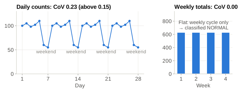
Day by day the series looks volatile. Summed by week it is perfectly flat, so the “anomaly” was just the weekly cycle.

2.3 Categorize the trend

Each series ends up in one of four states: UP, DOWN, NORMAL, or DISAPPEARING.

stateDiagram-v2
    [*] --> NormalData : Abs(Coefficient) < Threshold
    [*] --> TrendData : Abs(Coefficient) >= Threshold

    TrendData --> UP : Slope > 0
    TrendData --> DOWN : Slope < 0

    DOWN --> DISAPPEARING : Last value < 10% Avg

    UP --> NORMAL : Cov < 0.15 (Filter)
    DOWN --> NORMAL : Cov < 0.15 (Filter)

• Scale-aware thresholds. Sources are bucketed by volume (for example TINY, SMALL, MEDIUM, LARGE). Small sources are naturally noisy, so they need a larger trend coefficient before being flagged.
• Disappearing data. If the latest value drops to 0, or below 10% of the historical average, the series is flagged as DISAPPEARING regardless of the regression. This catches broken upstream feeds fast.

def classify(daily_counts, coef_threshold=0.02):
    values = np.asarray(daily_counts, dtype=float)
    avg = values.mean()
    if avg > 0 and values[-1] < 0.1 * avg:
        return "DISAPPEARING"
    coef = trend_coefficient(values)
    if abs(coef) < coef_threshold or is_cyclical_noise(values):
        return "NORMAL"
    return "UP" if coef > 0 else "DOWN"

In production, coef_threshold comes from the source’s volume bucket instead of a single constant.

Here is what each state looks like, with the regression line from step 2.1 overlaid. All four series were classified by the code above:

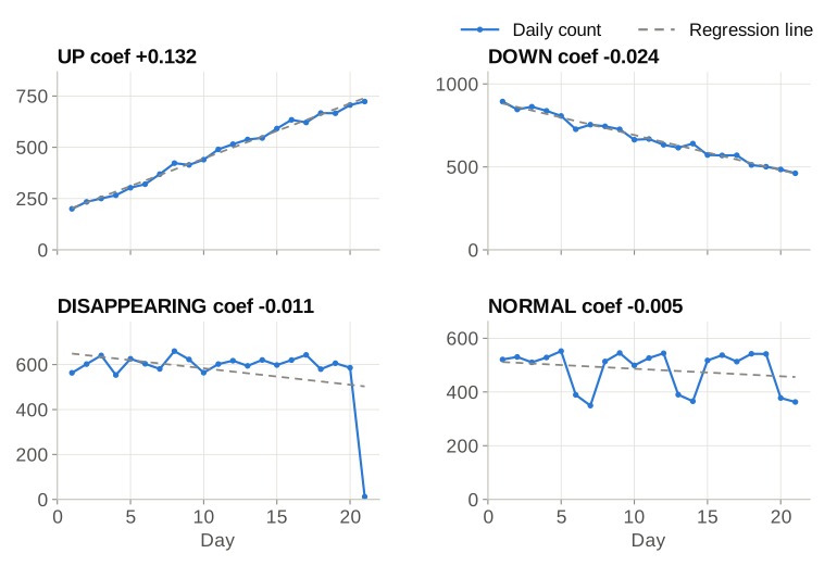
DISAPPEARING is caught by the last-value check even though its regression slope is small. NORMAL has visible dips, but they are the weekly cycle that step 2.2 filters out.

2.4 Secondary filtering with business logic

A final rejector removes flags that are technically trends but not worth a human’s time:

• Low volume: series with a very low average or too few daily counts are dropped.
• Distribution checks: if the first and second halves of the timeline have similar sums, or the recent average is close to the historical mean, the “trend” is likely noise.
• Median checks: if points are spread evenly above and below the median, that usually means random noise, not a structural shift.

3. ID pattern analysis

IDs such as order numbers are what tie records together across systems, so a wrongly extracted ID breaks joins silently. To find bad IDs without a hand-written rule per merchant, the framework converts every ID into a pattern: each run of digits or letters becomes a sized character class.

import re
from collections import Counter, defaultdict


def id_to_pattern(value):
    def repl(m):
        run = m.group()
        if run.isdigit():
            return f"[0-9]{{{len(run)}}}"
        if run.isalpha():
            return f"[A-Za-z]{{{len(run)}}}"
        return re.escape(run)

    return re.sub(r"[0-9]+|[A-Za-z]+|[^0-9A-Za-z]+", repl, value)


def summarize_patterns(ids, samples_per_pattern=3):
    counts = Counter()
    samples = defaultdict(list)
    for value in ids:
        pattern = id_to_pattern(value)
        counts[pattern] += 1
        if len(samples[pattern]) < samples_per_pattern:
            samples[pattern].append(value)
    return [(p, n, samples[p]) for p, n in counts.most_common()]

113-1234567 becomes [0-9]{3}\-[0-9]{7}. Group a day’s IDs by pattern, keep a few samples of each, and sort by frequency. The common patterns are the valid formats. The rare ones, with a handful of samples next to them, are where tagging errors hide, and a reviewer can scan them in minutes.

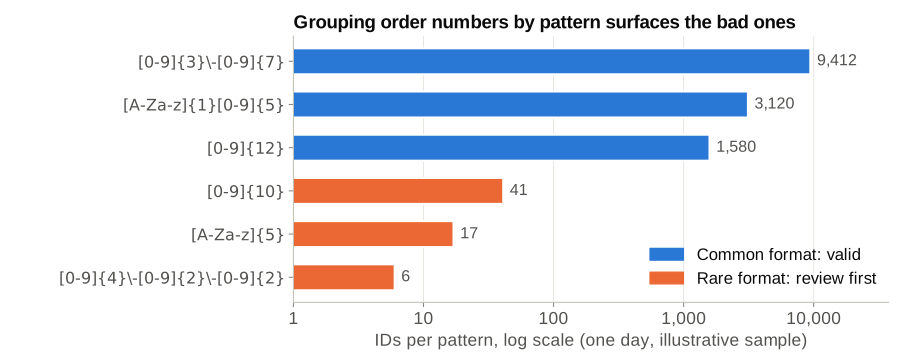
In this sample, the three rare patterns turn out to be phone numbers ([0-9]{10}), the word “Total” ([A-Za-z]{5}), and dates, all extracted into the order-number field by mistake. Reviewing 3 patterns is much faster than reviewing 64 bad records one by one. As patterns are confirmed valid or invalid, the list is refined to cover the majority of formats.

4. False alarm control

With hundreds of rules running daily, raw output is far too noisy to hand to reviewers. False alarm control runs in stages:

sequenceDiagram
    participant Raw as Raw Candidates
    participant Rule as Rule Filter (T)
    participant LLM as LLM / Similarity Filter (T+1)
    participant Rep as Final Reports

    Raw->>Rule: Pre-filter Phase
    Rule->>LLM: Pass tricky cases
    LLM-->>Rep: Verify similarity & context
    Rep-->>Rule: Feedback loop

• Rule pre-filtering caps the daily review sample size and skips known false-positive patterns.
• Similarity scoring compares each new candidate to the history of confirmed false alarms using the Levenshtein ratio. Anything close enough to a known false alarm is dropped:

from rapidfuzz.distance import Levenshtein


def looks_like_known_false_alarm(candidate, known_false_alarms, min_similarity=0.9):
    return any(
        Levenshtein.normalized_similarity(candidate, known) >= min_similarity
        for known in known_false_alarms
    )

• LLM filter. For tricky fields like order numbers, the remaining candidates go to a large language model. It gets the extracted value and the surrounding context and is asked whether the value is a real order number or noise (a phone number, a tracking ID, a date). This handles the ambiguous cases that regex can’t, at a fraction of the cost of human review.

The feedback loop matters as much as the filters. Every reviewer decision goes back into the known-false-alarm history and the rule pre-filters, so the system gets quieter over time instead of noisier.

What’s next

• Tighter LLM integration: combining regex candidates with LLM prompts for higher precision and less manual review.
• Broader monitoring: joining timeline data with wider business metrics to explain why a trend changed, not just that it changed.
• Self-serve platform: moving from fixed daily reports to a platform where data owners configure their own rules and thresholds.

Takeaways

• Use rules for known error classes. They’re cheap and explainable.
• Use trend detection for slow drifts that no single-record rule will catch, but invest most of the effort in filtering out normal variation.
• Turn free-form IDs into patterns to review formats instead of records.
• Treat false alarm control as a first-class component, with a feedback loop. Reviewer trust is what keeps a DQ system alive.

More from PipePrompt

• Kubernetes Scale-Down Was Eating Our Messages: Finding the Missing 0.01%

  Oct 19, 2026 · kubernetes, redis, python, etl, data quality

  An email ETL pipeline lost 10-odd messages per 100,000: pods killed mid-message on scale-down. The fix: a graceful exit plus a fallback queue.

• Migrating Production Spark Pipelines off Databricks: What Broke, and How We Proved the Data Matched

  Oct 13, 2026 · databricks, spark, migration, iceberg, data engineering, ai

  Moving dozens of Spark pipelines off Databricks: silent SQL translation bugs, hidden state, stale inputs, hash-based parity checks, and how AI helped.

• How MapReduce Works: From Hadoop Word Count to GROUP BY in Spark SQL

  Oct 11, 2026 · hadoop, mapreduce, spark, data engineering, databricks

  How Hadoop MapReduce works, with diagrams, a runnable word count, and how a GROUP BY on Databricks or WeData turns into map, shuffle and reduce.